The Hypothesis

In Part A, we compared four embedding models using three hand-crafted tests on 56 labeled entries and declared Azure OpenAI the winner. But the conclusion rests on thin evidence:

• 56 entries out of 16,282 — just 0.3% of the data
• 9 entities chosen specifically because they’re ambiguous English words (rock, honor, ruin)
• One threshold (0.7) for discovery evaluation, chosen by gut feel

The hypothesis of this post is straightforward: a proper evaluation on all available labeled data will tell a different story than a small hand-curated test set. We suspect:

1. Models that struggle on adversarial disambiguation (Gemini) might excel at the broader task of ranking relevant entries above irrelevant ones
2. The “best model” depends heavily on what you’re measuring — disambiguation accuracy, ranking quality, or graph reconstruction fidelity
3. F1 scores will be much lower at scale, and understanding why will reveal fundamental limits of embedding-based entity tagging

To test this, we built a cross-validation framework that evaluates every model on every tagged entry — not just the 56 we hand-picked.

---

The Question We’re Really Asking

Here’s the core task: given 622 entities and 16,282 WoB entries, can we take an entry that was not explicitly tagged with an entity and correctly predict whether it’s about that entity?

The Arcanum curators already tagged 7,813 entries with at least one entity. That’s our ground truth. We’ll hide some of those tags, try to predict them using embedding similarity, and measure how well we do.

Building a Validation Framework

Why Cross-Validation?

If you train a model on all 7,813 tagged entries and then test it on those same entries, you’ll get great numbers that mean nothing. The model has already “seen” the answers. This is called data leakage.

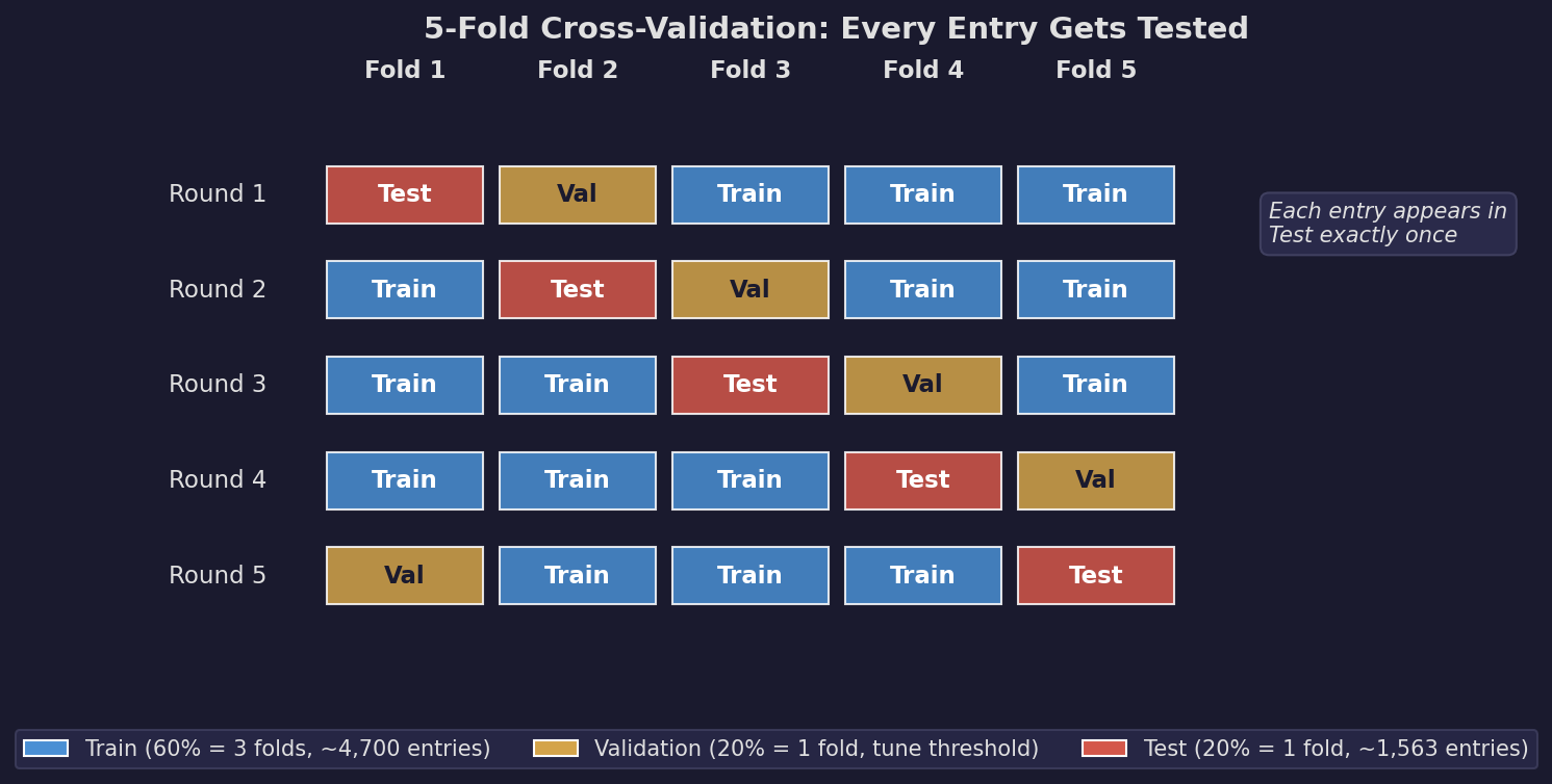
K-fold cross-validation solves this by splitting the data into K equally-sized groups (folds). For each round, you train on K-2 folds, use 1 fold to tune your threshold (validation), and test on the remaining fold. You rotate which fold is the test set and average the results.

Fold 1: [Train] [Train] [Train] [Val  ] [Test ]
Fold 2: [Test ] [Train] [Train] [Train] [Val  ]
Fold 3: [Val  ] [Test ] [Train] [Train] [Train]
Fold 4: [Train] [Val  ] [Test ] [Train] [Train]
Fold 5: [Train] [Train] [Val  ] [Test ] [Train]

We used K=5, giving us 5 rounds. Each entry appears in the test set exactly once. The three-way split (train/val/test) is important: the validation fold prevents us from implicitly overfitting the threshold to the test data.

The Stratification Problem

There’s a wrinkle. If you split randomly, a rare entity like “sja-anat” (mentioned in 3 entries) might end up entirely in one fold. Then when that fold is the test set, no training data exists for sja-anat, and when it’s a training fold, no test data exists. Either way, you can’t evaluate that entity.

Stratified splitting ensures every entity appears proportionally in every fold. For multi-label data (entries can have multiple entity tags), this is non-trivial. We use iterative stratification: entries are assigned to folds one at a time, starting with the rarest entities first, always placing each entry into the fold that most needs representation for that entry’s entities.

Here are the fold sizes we got: [1563, 1563, 1562, 1562, 1563] — nearly perfectly balanced.

What We Measure

Tag-level metrics tell us how well the model predicts individual entity-entry associations:

• Tag F1: The harmonic mean of precision and recall, averaged across all entities. (Same metric as Part A, but measured across 622 entities instead of 9.)
• Mean Average Precision (MAP): For each entity, rank all entries by their similarity score and check whether the truly-tagged entries appear near the top. MAP rewards models that rank relevant entries above irrelevant ones, regardless of what threshold you pick. A MAP of 1.0 means every entity’s truly-tagged entries rank above all non-tagged entries.

Edge-level metrics tell us how well the predicted tags reconstruct the knowledge graph:

• Edge F1: Two entities share an edge when they co-occur in the same entry. Using predicted tags, do we recover the same edges as the ground truth?
• Novel edges: How many edges appear in the predicted graph that don’t exist in the ground truth? This measures whether the model discovers genuine new connections vs. hallucinating relationships.
• Weight correlation: Do the predicted edge weights (co-occurrence counts) correlate with the true weights? A Spearman correlation of 1.0 means the model perfectly ranks which entity pairs are most strongly connected.

How Entity Representations Work

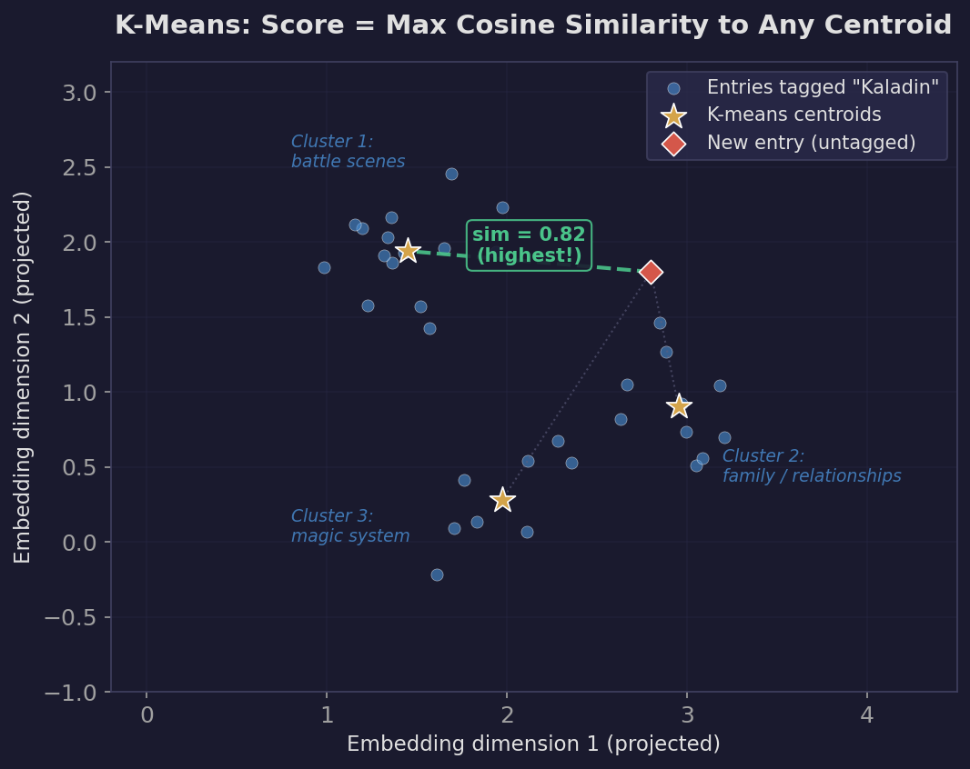
For each entity, we collect the embeddings of all training entries tagged with that entity and compute up to 3 k-means centroids. Why multiple centroids? Because an entity like “kaladin” is discussed in different contexts — battle scenes, family relationships, magic system mechanics. A single centroid (the average of all Kaladin entries) blurs these distinct clusters together. Three centroids can capture separate “modes” of discussion.

To score a new entry against an entity, we compute the cosine similarity between the entry’s embedding and each of the entity’s centroids, then take the maximum. If any centroid is a close match, the entry is likely about that entity.

We also tried more sophisticated representation methods:

Method	How it works	Parameters
K-means (1-3 centroids)	Cluster entity entries, score via max cosine similarity to nearest centroid	1-3 centroids based on sample count
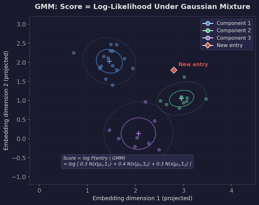
GMM diagonal	Gaussian Mixture Model with diagonal covariance on PCA-reduced embeddings, scored by log-likelihood	BIC-selected components, 100-dim PCA
GMM full	GMM with full covariance, captures feature correlations	BIC-selected components, 100-dim PCA
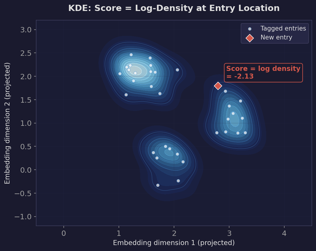
KDE	Kernel density estimation, non-parametric density	Silverman bandwidth

A Gaussian Mixture Model fits multiple elliptical Gaussian distributions to the data. Each component can have its own shape and orientation, capturing clusters that aren’t spherical. The score for a new entry is its log-likelihood under the mixture — how probable the entry is according to the learned density.

Kernel Density Estimation takes a different approach entirely. Instead of fitting parametric distributions, it places a small Gaussian “bump” centered on every training point and sums them up into a smooth density surface. The score for a new entry is the log-density at its location — higher in regions where many training entries are nearby.

The Results

Model Comparison (k-means representation)

Config	Tag F1	MAP	Threshold	Edge F1	Edge Recall	Novel Edges
Gemini	0.460	0.777	0.85	0.302	1.000	771
Cohere	0.401	0.731	0.69	0.398	1.000	886
Azure OpenAI	0.360	0.728	0.70	0.100	1.000	2,970
Voyage	0.276	0.699	0.70	0.076	1.000	3,992

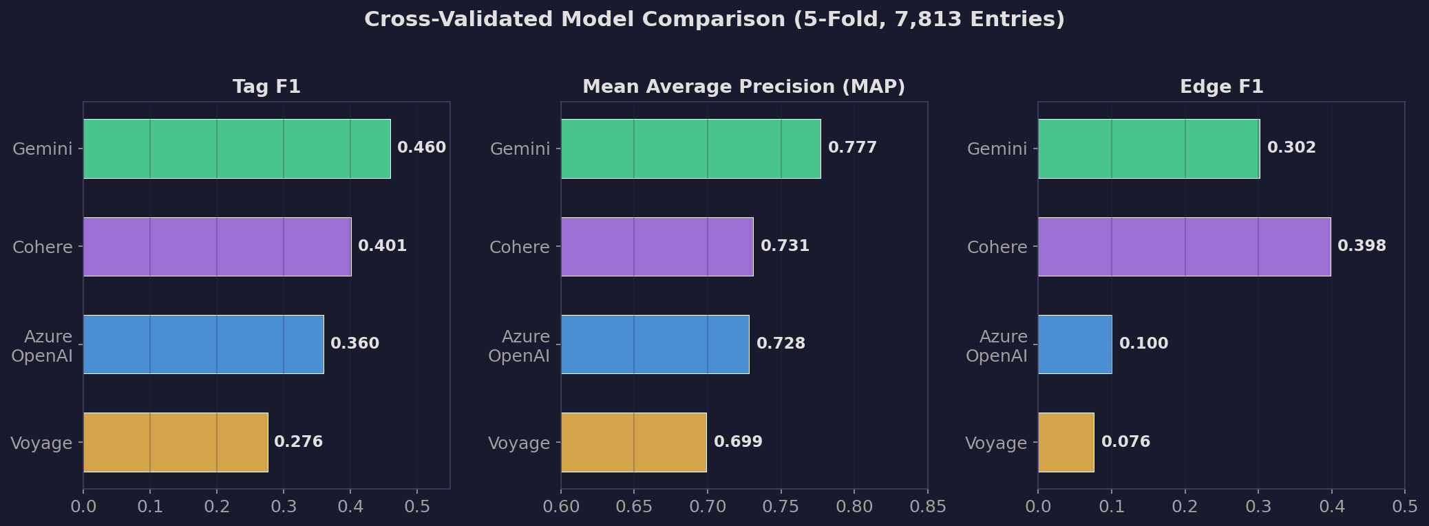
Gemini leads. Tag F1 of 0.460 and MAP of 0.777, both meaningfully ahead of the other models.

This directly contradicts Part A, where Gemini performed worst on disambiguation accuracy. What happened?

Why the Results Flipped

Part A’s 56-entry test set was specifically designed for disambiguation — telling “Rock the character” from “rock the noun.” This is a narrow, adversarial task where Gemini’s compressed similarity space works against it (everything scores above 0.7, so threshold-based classification fails).

The full validation tests something different: across 7,813 entries and 622 entities, can the model rank relevant entries above irrelevant ones? Gemini’s MAP of 0.777 means that on average, if you sorted all entries by their similarity to an entity, 77.7% of the time, a truly-tagged entry would rank above a non-tagged entry. Gemini’s compressed score range doesn’t matter here because MAP evaluates ranking, not thresholding.

The optimal threshold also tells a story. Gemini’s threshold is 0.85, while Azure OpenAI’s is 0.70. This confirms what Part A showed: Gemini’s scores are pushed up, so you need a higher cutoff. But the validation framework automatically tunes this per-fold, so the compression is compensated for.

Why F1 = 0.46 Is Not Bad

An F1 of 0.46 sounds terrible compared to Part A’s F1 of 0.93. But these are measuring fundamentally different things:

Part A: 56 entries, 9 entities, hand-picked for clear-cut answers. Each entry was chosen because a human could confidently say “yes, this is about Rock the character” or “no, this is about literal rock.”

Part B: 7,813 entries, 622 entities, no curation. This includes entries where the “right” answer is genuinely ambiguous.

Here’s a concrete example. Consider Kaladin Stormblessed from the Stormlight Archive:

False positive (predicted Kaladin, but not explicitly tagged):

“Tarah - what happened to her? […] She plays a small part.”

Similarity score: 0.751

Tarah is Kaladin’s love interest who appears briefly in Words of Radiance. An entry about Tarah is semantically very close to Kaladin’s cluster because the conversation context involves Kaladin’s relationships. The model says “this is about Kaladin” and is arguably correct — the entry is about a character whose only significance is through Kaladin. But the Arcanum curators tagged it only with “Tarah,” not “Kaladin.” The model gets penalized for a prediction that a human might agree with.

Another false positive:

“At the end of Rhythm of War, Adolin meets Dalinar after the contest of champions - but we don’t get to see it…”

Similarity score: 0.715

Adolin and Dalinar are Kaladin’s closest allies. This entry discusses a scene Kaladin was directly involved in. Again, the model’s “wrong” prediction is semantically reasonable — but the curators only tagged the entry with Adolin and Dalinar.

False negative (tagged Kaladin, but model scored it low):

“Are Lirin and Hesina Kaladin’s biological parents? Yes.”

Similarity score: 0.498

This entry is short and factual. It mentions Kaladin by name but has almost no semantic content — no discussion of battles, magic, or character arcs that would push it toward Kaladin’s cluster center. The model misses it because there’s not enough signal in four words to match the rich representation built from hundreds of Kaladin-related entries.

This is the fundamental tension. High-similarity false positives are entries that discuss Kaladin-adjacent topics in Kaladin-like language. Low-similarity false negatives are entries that name-drop Kaladin without discussing him substantively. A keyword matcher would catch the false negatives perfectly and miss the false positives. An embedding model does the opposite. F1 = 0.46 reflects a genuine boundary problem, not a model failure.

The Sparsity Factor

The entity tag distribution also constrains what F1 can achieve:

Entries per entity	Number of entities
1	107
2	68
3-5	119
6-10	83
11+	245

107 entities have only a single tagged entry. After the 60/20/20 train/val/test split, a single-entry entity has its one example in training, leaving zero entries in the test set to evaluate against (or vice versa). The model literally cannot be right or wrong for these entities — they contribute noise to the average.

Entries average only 1.6 tags each, and 4,572 entries (58%) have exactly one tag. This means most entries contribute to only one entity’s score, making the evaluation inherently sparse.

Why K-Means Beats Everything Else

We also tested three more sophisticated representation methods. Here are the results on Azure OpenAI:

Method	Tag F1	MAP	Notes
K-means (1-3 centroids)	0.360	0.728	Simple, works
GMM diagonal (PCA to 100-d)	0.042	—	Barely above random
GMM full (PCA to 100-d)	0.012	—	Worse than random

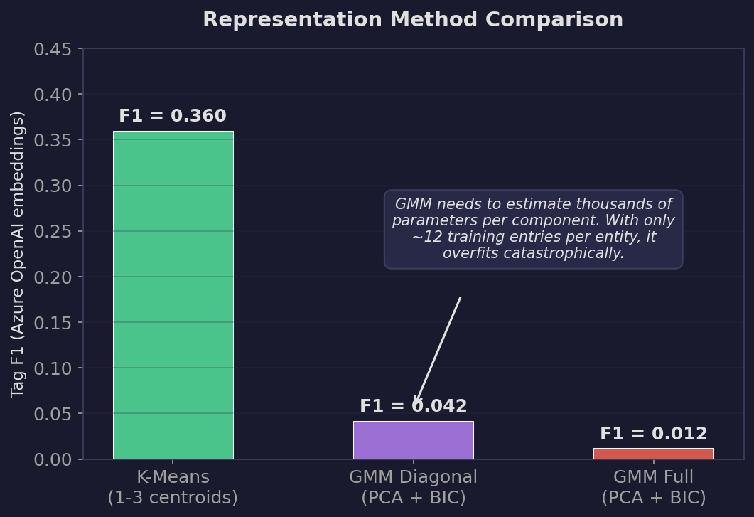
K-means wins by a huge margin. Why?

The bias-variance tradeoff. K-means has high bias (it assumes entities are spherical clusters) but low variance (it only needs to estimate 1-3 centroids, which requires fitting very few parameters). GMM has lower bias (it can model elliptical clusters with varying shapes) but much higher variance — a diagonal covariance matrix in 100 dimensions has 100 variance parameters per component, and a full covariance matrix has 5,050 parameters per component.

The median entity has about 12 tagged entries. Fitting 5,050 parameters from 12 data points is like fitting a degree-50 polynomial to 12 points — the model has far more capacity than the data can constrain, so it memorizes the training data instead of learning the underlying pattern. K-means fitting 3 centroid positions (3 x 3072 parameters, but on a normalized sphere the effective dimensionality is much lower) is far better-constrained.

We applied PCA reduction to 100 dimensions before fitting GMM to mitigate this, but even 100 dimensions was too many for the sample sizes we have. The fundamental problem is: entity representation is a few-shot learning problem, and simpler models win in few-shot regimes.

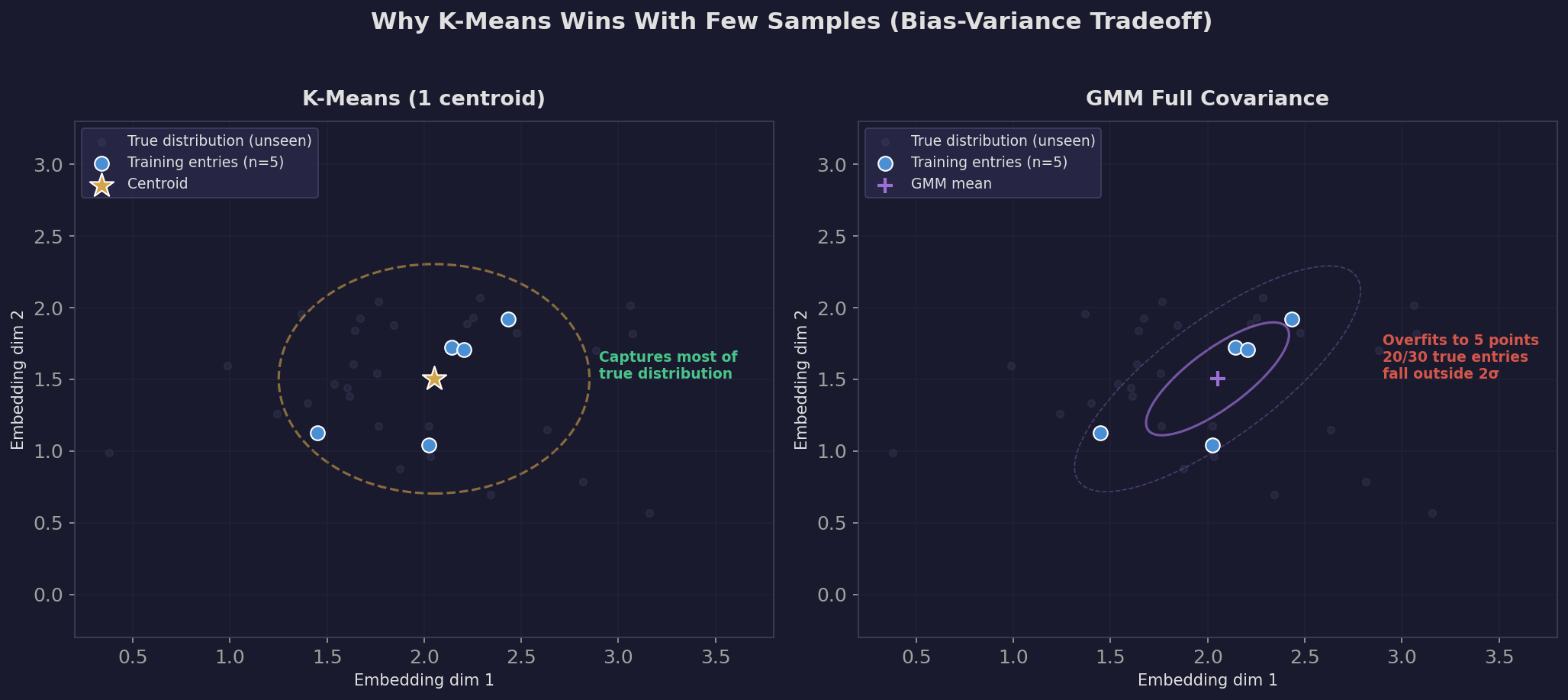
The plot below shows this visually. With only 5 training entries, k-means places a single centroid at their average — a broad, forgiving representation that captures most of the true distribution. GMM fits a tight ellipse around those 5 points, and most of the actual entity entries (shown as faint dots) fall outside its 2-sigma boundary.

Edge-Level Metrics: What They Add

The edge-level metrics tell a complementary story. Edge recall is 1.0 for every model — meaning every edge in the ground-truth graph also appears in the predicted graph. That’s because the predicted graph includes both explicitly tagged entries and implicitly tagged entries, so it’s a superset of the ground truth.

The more informative metric is edge F1, which penalizes models that predict too many edges. Cohere leads here (0.398) because it’s conservative — its threshold produces fewer implicit tags, so fewer spurious edges. Azure OpenAI’s edge F1 of 0.100 with 2,970 novel edges means most of its predicted edges don’t exist in the ground truth. But are they wrong, or are they genuine connections the curators missed? This is the discovery-vs-noise tradeoff we saw in Part A.

Weight correlation tells us whether the model gets the relative strength of connections right. Cohere leads (0.590), meaning the entity pairs it predicts to be most strongly connected are roughly the same pairs that are most connected in the ground truth. Azure OpenAI (0.418) and Gemini (0.530) are in the middle. Voyage (0.356) struggles most — consistent with its weaker tag-level performance.

What We Should Try Next

1. Hybrid scoring. Combine embedding similarity with keyword matching. The embedding model catches semantic connections (Tarah and Kaladin), while keyword matching catches name-drops in short entries (“Are Lirin and Hesina Kaladin’s parents? Yes.”). A simple weighted sum of the two scores might push F1 significantly higher.

2. Entity-specific thresholds. Currently every entity uses the same threshold. But “kaladin” (328 tagged entries) and “sja-anat” (3 tagged entries) have very different score distributions. Per-entity threshold tuning on the validation fold could improve precision for well-represented entities without sacrificing recall for rare ones.

3. Multi-prototype calibration. We use 1-3 centroids per entity based on sample count, but we never evaluated whether this was optimal. Sweeping the number of centroids per entity alongside the threshold could reveal that some entities benefit from more granular representations.

4. Cross-encoder reranking. Bi-encoder similarity (what we’re doing now) is fast but coarse. A cross-encoder takes the entry text and entity name as a pair and produces a more nuanced relevance score. Using bi-encoder similarity as a first-pass filter (top 50 entities per entry), then reranking with a cross-encoder, could improve precision substantially.

5. Fine-tuning on the domain. All four models are general-purpose embedding models trained on broad web data. Fine-tuning on the Cosmere corpus — even with a simple contrastive loss using the existing explicit tags as positive pairs — would teach the model domain-specific semantics like “Tarah is a minor Kaladin-related character.”

6. Better evaluation of novel edges. Our framework penalizes novel edges as false positives, but many of them represent genuine connections the curators missed. An evaluation that samples novel edges for human review would give a fairer picture of discovery power.

The Takeaway

Part A told us Azure OpenAI was the best model. Part B, using 139x more data and rigorous cross-validation, tells us Gemini leads on tag prediction quality (F1 = 0.460, MAP = 0.777) while Cohere leads on edge reconstruction fidelity (Edge F1 = 0.398, weight correlation = 0.590).

Neither answer is “right” in isolation. Part A measured disambiguation ability on adversarial examples. Part B measured broad prediction accuracy across the entire entity space. The choice of model depends on what you’re optimizing for — and the validation framework lets you measure that precisely instead of guessing.

The more interesting finding is that F1 = 0.46 is not a failure of the model. It’s a reflection of the fundamental gap between human tagging conventions (name-drop = tag) and semantic similarity (discussing someone’s love interest counts as “about” them). Understanding why a metric is low matters more than the number itself.